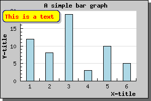
Figure 1: Adding a single text string in the upper left corner [src]
To add text you have to create one or more instances of the Text() object and then add the text object to the graph with the AddText() method.
The position of these text boxes are given as fraction of the width and height of the graph. When you are positioning these text boxes you might also choose what part of the text box should be considered the anchor point for the position you specify.
By default the anchor point is the upper left corner of the bounding box for the text.
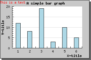
To show some ways of positioning the text we use a very simple bar
graph not to distract from the text. We first just add a single text
line with most of the settings their default value by adding the
following lines to the graph
 $txt=new Text("This is a text");

$txt->Pos(0,0);

$txt->SetColor("red");

$graph->AddText($txt);
The result is shown below.
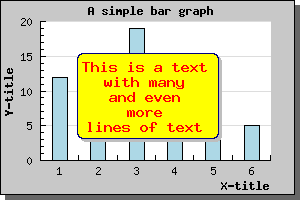
Not too exiting. Let's make it more interesting by having a background color, using larger fonts and framing the text box and adding a drop shadow to the text box by using the methods SetBox() and SetBox()
That's better. Now we get some attention. If you want to add a text with several lines you just need to separate the lines with a newline ('\n' character). The default paragraph alignment is left edge but you can also use right and center alignment.
As an illustration let's add a couple of more lines to the previous text, center the text box in the middle of the graph and also use centered paragraph alignment for the text. To adjust the paragraph alignment of the text you have to use the Text::ParagraphAlign()
Of course there is no limit to the number of text string you can add to the graph.
From version 1.12 it is also possible to add text strings to a graph using the scale coordinates instead. This is accomplished by using the Text::SetScalePos() Which is completely analogue to SetPos() with the only difference that the positions given are interpretated as scale values instead of fractions of the width and height.
The only thing you need to think of is that you probably want to add some extra margin to make room for the titles (using Graph::SetMargin() )
The individual positioning of these titles are done automatically and will adjust to the font size being used.
If you for, esthetic reasons, would like increase the distance from the top where the title is positioned (or the intra distance between title and sub title) you can use the Text::SetMargin() method. For example the line
$graph->title->SetMargin(20);
will set the distance between the top of the title string and the top of the graph to 20 pixels. If you instead call the SetMargin() method for the subtitle it will adjust the distance between the top of the subtitle and the bottom of the title.
The titles will be positioned at the top and be centered in the graph. Each of these titles may have multiple lines each separated by a "\n" (newline) character. By default the paragraph alignment for each title is centered but may of course be changed (using the ParagraphAlign()) method.
Each graph can also have a footer. This footer is actually three footers. Left, center and right. The 'left' footer is aligned to the left, the 'center' at the bottom center and the right to the right.
Each of these three positions is a standard Text object which means you can change color, font and size as you please individually on each of these footer positions.
You access the footer through the Graph::footer property as the following example shows
 $graph->footer->left->Set("(C) 2002
 KXY");

$graph->footer->center->Set("CONFIDENTIAL");

$graph->footer->center->SetColor("red");

$graph->footer->center->SetFont(FF_FONT2,FS_BOLD);

$graph->footer->right->Set("19 Aug 2002");You can access the tab using the 'tabtitle' property of the graph.
The following figure shows an example of how this can look.
As usual you have full freedom to specify font and colors for this type of title. Please see the class reference regarding GraphTabTitle() for more information.
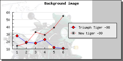
To use a specific image as the background you just have to use the method Graph::SetBackgroundImage() The arguments specify file-name, how the image should be positioned in the graph and finally the format of the image (if it is in JPG, PNG or GIF) format. If the format is specified as "auto" (the default) then the appropriate image format will be determined from the extension of the image file.
The file name is of course obvious but the second argument might not be. This arguments determine how the image should be copied onto the graph image. You can specify three different variants here
You might often find yourself wanting to use a background image as a "waterstamp". This usually means taking the original image, import it to some image editing program and then "bleaching" the color saturation, reducing the contrast and so on. Finally you save the modified image which you then use as a background image.
This whole process can be automatically accomplished in JpGraph by using the method Graph::AdjBackgroundImage() which allow you to adjust color saturation, brightness and contrast of the background image.
For example, in the image below I have used the settings
$graph->AdjBackgroundImage(...)
to achieve the "watercolor" effect to avoid the image being too intrusive in the graph.
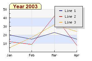
You specify a color gradient background by calling the Graph::SetBackgroundGradient() method. All details are available in the class reference (follow the link above). We finally give a quick example on what kind of effect you can achieve using this feature.
Finally we like to mention that in the "/utils/misc/" directory you will find a small utility script called "mkgrad.php". Running this script presents you with a UI that makes it a breeze to create a gradient image on it's own.
The UI for the utility is so obvious that we won't discuss it
further, we just show it below. The UI for the mkgrad.php utility
In the example below I have used this utility to get a more interesting plot area.
This callback function will get called with the current Y-value (for the plotmark) as it's argument. As return value the callback function must return an array containing three (possible null) values. The values returned must be
The callback must be a global function and is installed with a call to PlotMark::SetCallback()
So for example to install a callback that changes the fill color for all marks with a (Y) value higher than 90 you could add the lines
90) $fcolor="red" else $fcolor=""; return array("","",$fcolor); } ... $plot->mark->SetCallback("MarkCallback"); ...'; ShowCodeSnippet($t); ?>
As you can see in the above example we have left some of the return values blank. Doing this will just ignore any change of these value and use the global settings for the plotmarks.
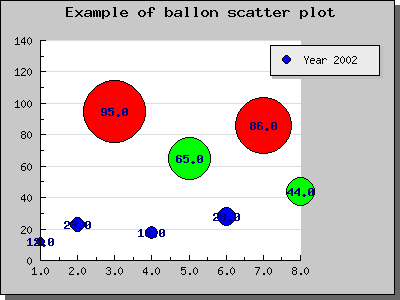
If you also let the (Y) value affect the size of the plot marks you can get what is sometimes known as a "balloon plot". The example below is basically a scatter plot that uses filled circles to mark the points. A format callback is then used to change the color and size depending on the Y-value for each plot.
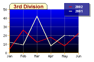
The slight complication with general rotation is that the margins also rotates, this means that if you rotate a graph 90 degrees the left margin in the image was originally the bottom margin. In additional by default the center of the rotation is the center of the plot area and not the entire image (if all the margins are symmetrical then they will of course coincide). This means that depending on your margin the center of the rotation will move. You can read more about this and how to manually set the center for rotation in the section about rotation, 10.2
This is just a slight inconvenience which you have to take into account when you need to set an explicit margin with a call to Graph::SetMargin()
However, in order to make a rotation of 90 degrees much easier you can easily rotate a graph 90 degrees and set the correct margin with a call to Graph::Set90AndMargin() The parameter to this method lets you specify the margins as you will see them in the image without having to think of what becomes what after the rotation.
So, the only thing you need to do is call this method and then the graph will have been rotated 90 degrees.