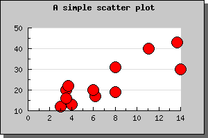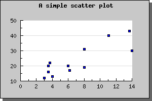
Figure 1: The simplest possible scatter plot [src]
Even though you would normally supply X-coordinates it is still perfectly possible to use a text-scale for X-coordinates to just enumerate the points. This is especially useful when using the "Impuls" type of scatter plot as is shown below.
Scatter pots are created by including the jpgraph extension "jpgraph_scatter.php" and then creating an instance of plot type of ScatterPlot(). To specify the mark you want to use you access the mark with the instance variable "mark" in the scatter plot. The default is to use an unfilled small circle.
To create a scatter plot you will create an instance
A simple example using just default values will illustrate this
We can easily adjust the size and colors for the markers to get another effect as shown below
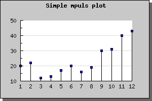
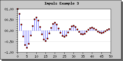
Another possible variant of scatter plot is impuls-scatter plots. This is a variant of normal scatter plot where each mark have a line from the mark to the Y=0 base line. To change a scatter plot into an impuls scatter plot you have to call the method SetImpuls() on the scatter plot.
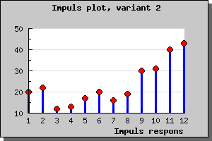
This type of plots are often used to illustrate signals in conjunction with digital signal processing. The following two examples illustrates simple use of impuls plots.
The next example shows how to modify the color and width of the impuls plot
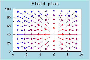
To create a field plot you create an instance of FieldPlot in the same way as you created a normal scatter plot. The arguments to this method are Y-coordinate, X-coordinate and angle. To specify a callback you use FieldPlot::SetCallback()
The following example (and code) illustrates the usage of the field plot type.
In addition to the parameters mentioned above you can also adjust both the general size of the arrow and also the specific size of the arrowhead. The arrow size is specified in pixels and the arrow head is specified as an integers between 0 and 10. These sizes are specified with a call to FieldPlot::arrow::SetSize()